I’ve broken this post up into two parts, the Math and the Implementation. You don’t need to understand the math to generate these patterns, but without the background, the code might look like magic. Understanding the math should hopefully bring some intuition to what exactly the parameters control, how to tweak them, and what to expect when combining multiple groups.

The Math

What is a wallpaper?

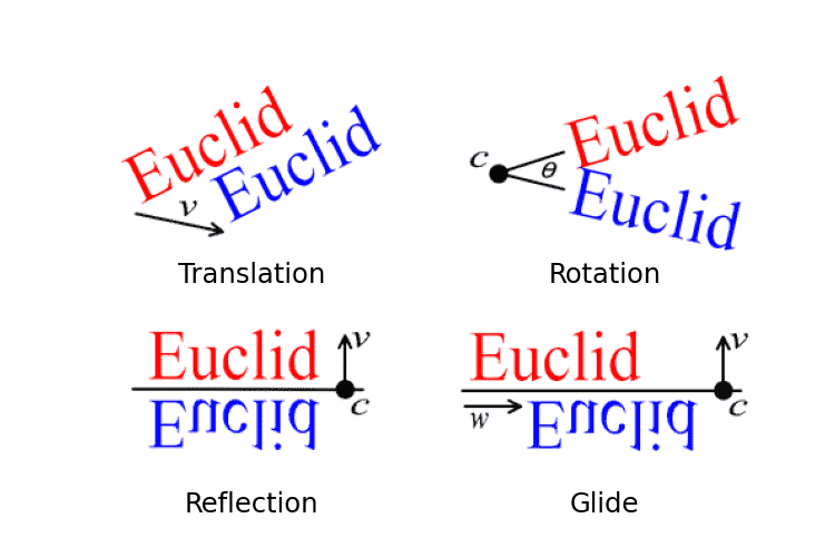
Formally, a wallpaper group is a type of topologically discrete group of isometries of the Euclidean plane that contains two linearly independent translations. In simpler terms, a wallpaper group is a collection of 2D patterns that can repeat themselves in two distinct directions. These wallpapers are categorized by their symmetry group type. These symmetry group types are built by combining four kinds of transformations, translations, rotations, reflections, and glide reflections. Wikipedia provides a nice overview of the 17 unique wallpaper groups that can be formed from these transformations of the plane.

These groups are able to construct an infinitely repeating pattern based off of a applying these four transformations to a single tile. Depending on the specific group, that tile can be triangular, square, rectangular, rhombic, or oblique (a parallelogram). The most basic example of this is the p1 group. The p1 group is constructed by translating any of the above tile shapes, excluding triangular, on both the horizontal and vertical axis. A real world example of this would be tiling a floor with single colored tiles.

The information about the constructions of can be captured in a cell diagram. Let’s look at the cell diagram for the p2 group to understand how we would want to read this.

The rectangle colored in yellow is called the fundamental domain – the smallest part of the pattern that is repeated. The diamonds on the edges of the rectangles represent points where the cell can be rotated 180 degrees about. The blue diamond in the center means that the upper rectangle should be the lower rectangle just flipped both left/right and up/down. If we were to translate this entire square to the right similar to p1, it would look as if we copied the lower rectangle without changing it directly to the right. The green rectangles capture that the upper rectangle would also copy over, which was 180 degrees rotated to the original. Similarly, if we were to translate the whole cell up and down, the red and pink diamonds capture how the rotational pattern is repeated.

If the math isn’t making it any easier to visualize these things, I’d recommend checking out this web app made by David Eck. It allows you to get a nice idea of what the symmetry types look like without having to learn how to read a cell structure diagram.

Turning Patterns into Images

Making wallpaper patterns usually means drawing out something as the fundamental cell and applying the needed transformations on that cell across the plane. This method allows for creating images that are reminiscent of M.C. Escher’s work with tessellations – this isn’t a coincidence as it was Escher’s own study of the 17 wallpaper groups that inspired his work with regular periodic tessellations.

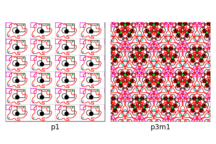
This method of construction unfortunately does become stale after some time, since at its core, the fundamental cells that are used to construct the pattern are easily identifiable, and arbitrary composition of wallpapers given the same base fundamental domain becomes very difficult given the constraints each group has on the fundamental domain.

Moving into the Continuous Domain

Frank A. Faris’s Creating Symmetry explores how to construct the wallpaper symmetries from a superposition of waves, instead of a collection of symmetric transformations. The book does a wonderful job of walking through how the eigenfunctions of the Laplacian of the wave equation can be constrained to require the symmetric invariances that categorize the wallpaper groups, along with how the lattices which translation is periodic can be constructed. If you want to really build an intuition about these things, the book is an invaluable resource.

To try to demystify the process as much as possible, hopefully giving some intuition to any parameters, each group can be a specific combination of the following parts.

1. The lattice vectors of the wave that shape the translations on the grid
   • General (parallelograms)
   • Rhombic (rhomuses)
   • Rectangular
   • Square
   • Hexagonal
2. A function over the lattice that generates ensures rotational symmetry
   • A single wave
   • A collection of 3 single waves that are constrained to 60 degree symmetry
   • A collection of 4 single waves that are constrained to 90 degree symmetry
3. A coefficient constraint that helps ensure any of the following
   • Reflective symmetry
   • Glide symmetry
   • Additional rotational symmetry

The Basic Building Block

The basic wave that we use is the function \( f \) that satisfies \(\frac{\partial^{2} u}{\partial t^{2}} = c^{2} \nabla u \) for a plane.

We’ll extend this two a lattice defined by lattice vectors \( X(z) \) and \( Y(z) \), where \( X(z) \) and \( Y(z) \) are linearly independent.

Any wallpaper pattern defined over the lattice specified by \( X \) and \( Y \) can be completely constructed from a linear combination of \( E_{n,m} \) waves.

The Lattices

The \( X \) and \( Y \) functions allow us to take points defined in a plane, where \(z = x + iy \), and map them onto a lattice defined by two vectors for a general use case.

General Lattice

The general lattice can be any two independent vectors. This will result in what parallelogram cells. We can construct \( X \) and \( Y \) for the general case with two vectors, \(1,\; \omega = \xi + i\eta \) with \( \eta \neq 0 \).

Rhombic Lattice

The rhombic lattice vectors are of the form \( \omega \pm bi \), with \(b \neq 0 \). These result in centered rhombus cells. \( X \) and \(Y \) are constructed for the rhombic lattice as follows.

Rectangular Lattice

The rectangular lattice is defined by vectors \(1, Li \), with \(L \neq 0 \). This will result in rectangular cells. \(X \) and \( Y \) are defined as follows

Square Lattice

The square lattice is the special case of the rectangular lattice where \( L=1 \), i.e.

Hexagonal Lattice

Finally, the hexagonal lattice is defined by the vectors \(1, \omega_{3} = \frac{-1 + i \sqrt{3}}{2} \), a special version of the general case resulting in hexagonal cells. \(X \) and \(Y \) are as follows

The Rotational Symmetry Constraints

Four Fold Symmetry

Given a base wave defined by \( E_{n,m}(z) \) defined on the square lattice, we can leverage the 90 degree symmetry of the lattice to find 3 other waves that interfere with each other in such a way that ensures 4 fold symmetry. Given the square lattice \( n, m \) can be thought of as the linear wavenumber of the \( x \) and \( y \) components of the wave respectively, i.e. \( \tilde{\nu_{x}} = \frac{1}{\lambda_{x}} \;, \tilde{\nu_{y}} = \frac{1}{\lambda_{y}} \).

Note, this wavenumber analogy holds for the other lattice definitions as well, however, instead of \( n, m \) corresponding to the wavenumbers in \( x \) and \( y \), they correspond to the wavenumbers across the \(X \) and \(Y \) components of the lattice. In the case of the square lattice, the \(X \) and \(Y \) components of the lattice are the \(x \) and \(y \) components of the plane.

To ensure four fold symmetry, of \( E_{n,m}(z) \), we can first add on a wave traveling in the exact opposite direction \( E_{-n, -m}(z) \). The result of combining these two waves is a mirroring of the original wave about the \( \langle n, m \rangle \) propagation direction. After that, since we have the advantage of the square lattice, we know that the vector orthogonal to the original vector can be found with a simple 90 degree rotation of the original vector. Given a vector \(\vec{a} = \langle a_{x}, a_{y} \rangle \) a 90 degree rotation can be simply expressed as \(\vec{a}^{\perp} = \langle -a_{y}, a_{x} \rangle \). Leveraging this on our original \( E_{n, m}(z) \) would mean that a wave propagating perpendicular would be expressed as \( E_{-m, n}(z) \). That similarly means that the wave the propagates perpendicular to the inverse wave is \( E_{-m, -n}(z) \). This means that we have 4 waves, all propagating at 90 degree angles to each other. This allows us to define a function to constrain a given \( n, m \) to four fold rotational symmetry as

Three Fold Symmetry

Similarly, to ensure three fold symmetry, we can leverage the fact that the hexagonal lattice’s basis vectors form a 120 degree angle between them to find 3 waves that all propagate at 120 degree angles to each other – yielding 3 fold symmetry.

The process for finding these vectors is similar to what we had to do for finding the vectors for four fold symmetry, except not as trivial as rotating the vector by 90 degrees in the plane. Given that we have a wave propagating at \( \langle n, m \rangle \) in the hexagonal lattice, we want to find vectors that form 120 degree and 240 degree angles in the \( x, y \) plane to \( \langle n, m \rangle \). I’ll leave the details of verifying that these hold to the reader, but the corresponding vectors are \( \langle m, -\left(n+m \right) \rangle \) and \( \langle -\left(n+m \right), n \rangle \). This allows us to define our three fold symmetry constraint in the hexagonal lattice as

The Additional Coefficient Constraints

If we were to not add anymore constraints to our wave constructions across the lattices, we’d only be able to be guaranteed to construct the p1, p4, and p3. The additional constraints are selected through a similar process to how the rotational symmetry constraints were defined, but targeting the specific reflection, rotational, and glide symmetries that categorize the rest of the wallpaper groups. I’m not going to go into the details of how these are selected, as doing so would require addressing each of the 14 remaining cases individually. The important note here, is that these coefficient constraints happen after any rotational symmetry constraints have been defined. So for wallpaper groups defined on the square and hexagonal lattices, these coefficients constrain \(S_{n,m} \) and \(W_{n, m} \) respectively, while for the rest of the lattices, \(E_{n, m} \) is constrained.

Putting it all together

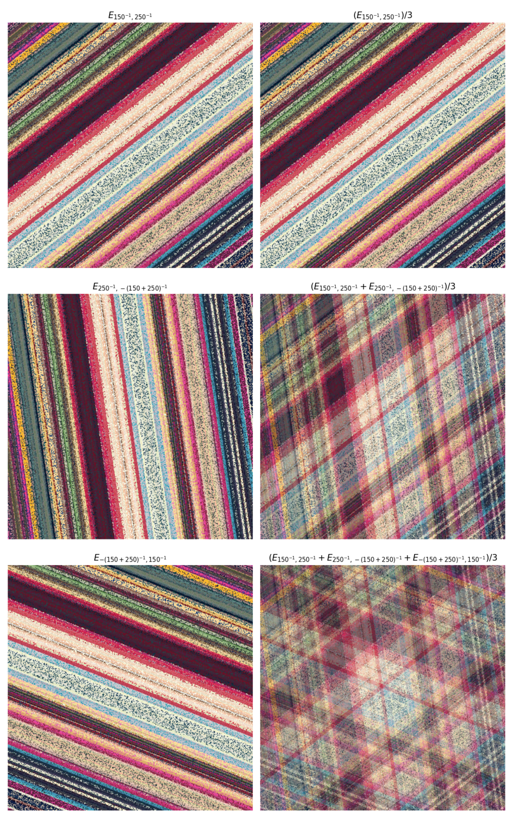
Each of the 17 groups can be defined by selecting a lattice \(X(z), Y(z) \) for the base \(E_{n,m}\), a symmetry constraint \(F_{n,m} \in \lbrace E_{n,m}, S_{n,m}, W_{n,m} \rbrace \) and coefficient constraints on \(a_{n, m} \). Given these criteria, a function \(f(z) \) can be defined which represents a function that represents a complex transformation that will produce the desired wallpaper symmetry.

The following table covers the criteria for creating a wallpaper function \( f(z) \) for each of the 17 wallpaper groups.

The Code

The table above contains the all the information needed to implement general purpose wallpaper functions. Translating these functions into Python takes care of the majority of the work needed to apply these wallpaper functions to arbitrary images. The only additional parts that we’ll need to define are how to initialize the array that we apply the wallpaper function to, and how to colormap the result of applying the wallpaper function.

Setup and Dependencies

The dependencies that I based this implementation around are:

1. numpy – For improved array handling
2. matplotlib – For image I/O
3. numba – For CUDA support

These can be installed as follows:

$ pip install numpy matplotlib numba

On top of this, we’ll be calling out to the math and cmath builtin modules. This leaves us with the following import cluster

import cmath
import math

import numba.cuda as cuda
import numpy as np
import matplotlib.pyplot as plt

numba.cuda requires a supported Nvidia GPU with an accessible CUDA installation on the system. The official installation instructions for this can be found here.

While I’ve written the rest of this section assuming that numba.cuda is available, the section below should give an outline of what would need to be adapted to implement this without GPU acceleration. If you do have access to numba.cuda, feel free to skip to the canvas initialization.

Following along without CUDA

If you’re looking to follow along and don’t have access to a system with an Nvidia GPU and CUDA installation, you have a couple of options.

You could choose to simply omit the @cuda.jit decorators, and then convert the logic of i, j = cuda.grid(2) to a nested loop. While this is the easy solution it comes with the downside of being in pure Python, meaning that this will likely be excruciatingly slow.

You could also change the @cuda.jit(device=True) decorators to @numba.jit decorators, and then any functions with @cuda.jit to @numba.jit(parallel=True) and change then make the following logic adaption:

i, j = cuda.grid(2)
if i < out.shape[0] and j < out.shape[1]:
    ...

To a set of nested loops on the indexes of the out array:

for i in range(out.shape[0]):
    for j in range(out.shape[1]):
        ...

In both cases, when actually calling the functions, the @numba.jit variants can directly passed the numpy arrays, and the gpu_* variants aren’t needed. As well, the [blocks_per_grid, threads_per_block] on the calls to the @cuda.jit functions are no longer needed either.

Initializing the Canvas

Our canvas will be a 2D array of complex numbers that range from \( -1\text{ to }1 \) on the x-axis, and \( -i\text{ to }i \) on the y-axis. We’ll make use of np.linspace to generate a 1D array of evenly spaced numbers for each axis and np.meshgrid to generate a evenly spaced 2D grid from the x and y axis arrays.

def make_complex_canvas(width : int, height : int) -> 'np.ndarray[np.complex]'
    if height > width:
        x = np.linspace(-1*width/height, 1*width/height, width)
        y = np.linspace(-1, 1, height)
    elif width > height:
        x = np.linspace(-1, 1, width)
        y = np.linspace(-1*height/width, 1*height/width, height)
    else:
        x = y = np.linspace(-1, 1, width)
    xx, yy = np.meshgrid(x, y)
    return xx + yy*1j

Implementing the Wallpaper Functions

The details for these functions can be found in the math section. Each of the 17 wallpaper functions have a unique combination of the lattice, \( F_{n, m} \), and coefficient constraints. We’re going to break this down into 3 parts:

1. Defining \(E_{n,m}\) functions for each lattice type
2. Defining the \(S_{n,m}\text{ and } W_{n,m}\) constraint functions
3. Defining a function for each wallpaper group that takes a single combination of \(a, n, m\) values and handles any coefficient constraints accordingly.

The \(E_{n,m}\) lattice functions

\( E_{n, m} \) will always take the form,

Since the choice of \(X, Y \) is dependent on the lattice, we’re going to define the functions that already propagate through \(X, Y\) into \(E_{n,m}\). The specifics of \(X, Y\) for each lattice type are defined in the math section

We’ll be decorating all of these functions with @cuda.jit(device=True) since we intend to call this function from within another cuda function. The device=True keyword in the decorator tells numba that this function is written to run directly on the GPU, and can be compiled as such.

@cuda.jit(device=True)
def Enm_general(z: complex, n: int, m: int, omega: complex) -> complex:
    return cmath.exp(2*cmath.pi*1j*(n*(z.real - omega.real*z.imag/omega.imag) + m*z.imag/omega.imag))

@cuda.jit(device=True)
def Enm_rhombic(z: complex, n: int, m: int, b: float) -> complex:
	return cmath.exp(2*cmath.pi*1j*(n*(z.real + z.imag/(2*b)) + m*(z.real - z.imag/(2*b))))

@cuda.jit(device=True)
def Enm_rectangular(z: complex, n: int, m: int, L : float) -> complex:
    return cmath.exp(2*cmath.pi*1j*(n*z.real + m*z.imag/L))

@cuda.jit(device=True)
def Enm_square(z: complex, n: int, m: int) -> complex:
    return cmath.exp(2*cmath.pi*1j*(n*z.real + m*z.imag))

@cuda.jit(device=True)
def Enm_hexagonal(z: complex, n: int, m: int) -> complex:
	return cmath.exp(2*cmath.pi*1j*(n*z.real + z.imag/math.sqrt(3)) + m*(2*z.imag/math.sqrt(3)))

Implementing \(S_{n, m}, W_{n, m}\)

The definitions of \(S_{n, m}, W_{n, m}\) can be found in the math section Just like the \(E_{n, m}\) implementations, these will also be decorated with @cuda.jit(device=True) since we intend on calling these from within another cuda function as well.

@cuda.jit(device=True)
def Snm(z: complex, n: int, m: int) -> complex:
    return (Enm_square(z, n, m) +
            Enm_square(z, m, -n) +
            Enm_square(z, -m, n) +
            Enm_square(z, -m, -n)) / 4

@cuda.jit(device=True)
def Wnm(z: complex, n: int, m: int) -> complex:
    return (Enm_hexagonal(z, n, m) +
            Enm_hexagonal(z, m, -(n+m)) +
            Enm_hexagonal(z, -(n+m), n)) / 3

Implementing the coefficient constraints

For each group that has coefficient constraints, we are going to enforce those constraints similar to how \(S_{n, m}, W_{n, m}\) enforce their symmetry, by returning the waves already averaged.

Again, these are all @cuda.jit(device=True) decorated since we intend on calling them from the cuda function that applies the mapping to the canvas.

@cuda.jit(device=True)
def p1(z: complex, n: int, m: int, omega: complex, a : complex) -> complex:
    return a*Enm_general(z, n, m, omega)

@cuda.jit(device=True)
def p2(z: complex, n: int, m: int, omega: complex, a : complex) -> complex:
    return a*(Enm_general(z, n, m, omega) +
              Enm_general(z, -n, -m, omega)) / 2

@cuda.jit(device=True)
def cm(z: complex, n: int, m: int, b: float, a: complex) -> complex:
    return a*(Enm_rhombic(z, n, m, b) +
              Enm_rhombic(z, m, n, b)) / 2

@cuda.jit(device=True)
def cmm(z: complex, n: int, m: int, b: float, a: complex) -> complex:
    return a*(Enm_rhombic(z, n, m, b) +
              Enm_rhombic(z, m, n, b) +
              Enm_rhombic(z, -m, -n, b) +
              Enm_rhombic(z, -n, -m, b)) / 4

@cuda.jit(device=True)
def pm(z: complex, n: int, m: int, L: float, a: complex) -> complex:
    return a*(Enm_rectangular(z, n, m, L) +
              Enm_rectangular(z, n, -m, L)) / 2

@cuda.jit(device=True)
def pg(z: complex, n: int, m: int, L: float, a: complex) -> complex:
    return a*(Enm_rectangular(z, n, m, L) +
              (-1)**n*Enm_rectangular(z, n, -m, L)) / 2

@cuda.jit(device=True)
def pmm(z: complex, n: int, m: int, L: float, a: complex) -> complex:
    return a*(Enm_rectangular(z, n, m, L) +
              Enm_rectangular(z, n, -m, L) +
              Enm_rectangular(z, -n, m, L) +
              Enm_rectangular(z, -n, -m, L)) / 4

@cuda.jit(device=True)
def pmg(z: complex, n: int, m: int, L: float, a: complex) -> complex:
    return a*(Enm_rectangular(z, n, m, L) +
              Enm_rectangular(z, -n, -m, L) +
              (-1)**n*Enm_rectangular(z, n, -m, L) +
              (-1)**n*Enm_rectangular(z, -n, m, L)) / 4

@cuda.jit(device=True)
def pmg(z: complex, n: int, m: int, L: float, a: complex) -> complex:
    return a*(Enm_rectangular(z, n, m, L) +
              Enm_rectangular(z, -n, -m, L) +
              (-1)**(n+m)*Enm_rectangular(z, n, -m, L) +
              (-1)**(n+m)*Enm_rectangular(z, -n, m, L)) / 4

@cuda.jit(device=True)
def p4(z: complex, n: int, m: int, a: complex) -> complex:
    return a*Snm(z, n, m)

@cuda.jit(device=True)
def p4m(z: complex, n: int, m: int, a: complex) -> complex:
    return a*(Snm(z, n, m) +
              Snm(z, m, n)) / 2

@cuda.jit(device=True)
def p4g(z: complex: n: int, m: int, a: complex) -> complex:
    return a*(Snm(z, n, m) +
              (-1)**(n+m)*Snm(z, m, n)) / 2

@cuda.jit(device=True)
def p3(z: complex, n: int, m: int, a: complex) -> complex:
    return a*Wnm(z, n, m)

@cuda.jit(device=True)
def p31m(z: complex, n: int, m: int, a: complex) -> complex:
    return a*(Wnm(z, n, m) +
              Wnm(z, m, n)) / 2

@cuda.jit(device=True)
def p3m1(z: complex, n: int, m: int, a: complex) -> complex:
    return a*(Wnm(z, n, m) +
              Wnm(z, -m, -n)) / 2

@cuda.jit(device=True)
def p6(z: complex, n: int, m: int, a: complex) -> complex:
    return a*(Wnm(z, n, m) +
              Wnm(z, -n, -m)) / 2

@cuda.jit(device=True)
def p6m(z: complex, n: int, m: int, a: complex) -> complex:
    return a*(Wnm(z, n, m) +
              Wnm(z, -n, -m) +
              Wnm(z, m, n) +
              Wnm(z, -m, -n)) / 4

Mapping a Wallpaper Function to the Canvas

Now we have everything in place that will allow us utilize any of the above 17 wallpaper groups in constructing what we wish to map. This is the @cuda.jit function that we are currently defining which would call out to our wallpaper functions.

An important thing to note here is that this function will be run parallel, meaning it should only update 1 value of the canvas at the time. This means that we won’t be iterating through the array, or operating on it in place. Instead, we’ll need to pass it an empty array which it can store the result in. To know which value we should be operating on, numba provides a cuda.grid method to internally tell us what the coordinates are of the current function call. Since this function will be operating on a 2D grid, we’ll call i, j = cuda.grid(2). Important to note, these i, j, just happen to be the coordinates of where in the GPU we are operating. Just because we’re operating at that i, j, doesn’t mean our data is defined at i, j, so we’ll need to check that we’re not out of bounds before doing anything.

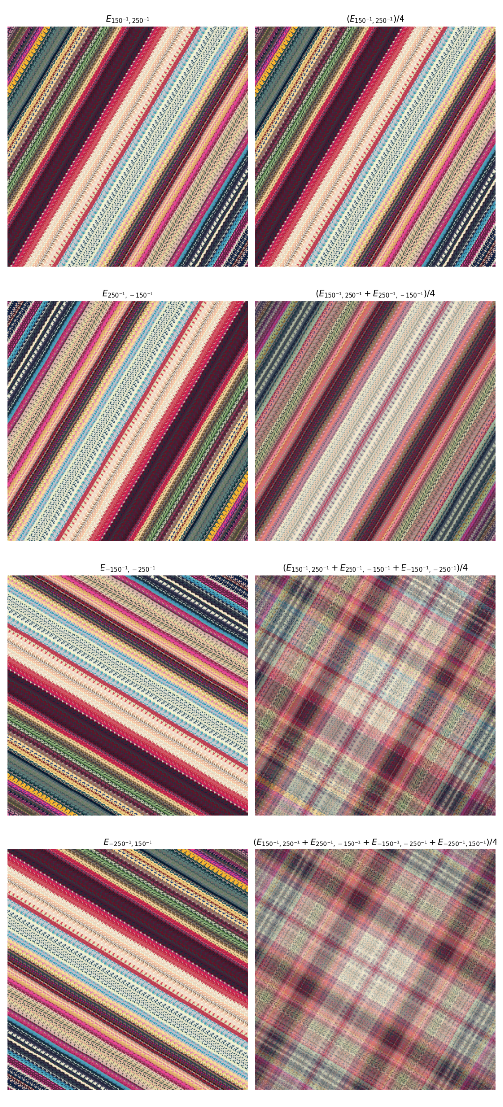
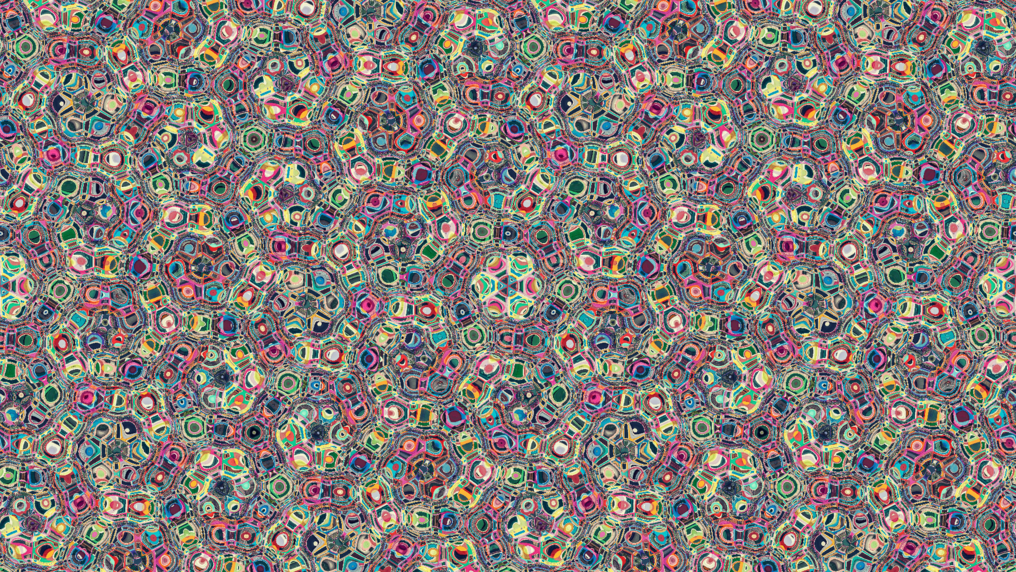
Let’s try an example where the wallpaper function is the result of adding together 2 p3 functions.

@cuda.jit
def example_wallpaper(out, canvas):
    i, j = cuda.grid(2)
    if i < out.shape[0] and j < out.shape[1]:
        val = canvas[i, j]
        out[i, j] = p3(val, 2, 4, 1/2) + p3(val, 5, 6, -1/2)

Colormapping the Canvas

After we apply our function, we’ll be left with the issue of how to turn a complex 2D array into an image. To do this, we’re going to define a function that uses an arbitrary image as the complex colormap for the array. We’ll do this by scaling the value of the array into the closest index we can on the image. We’ll map it so that the x coordinate of the image is scaled to the magnitude of the value, and the y coordinate of the image is scaled to the phase of the value.

@cuda.jit(device=True)
def scale_to_range(val, a, b):
    return (val - a) / (b - a)

@cuda.jit
def colormap_complex(out, data, img, xmin, xmax, ymin, ymax):
    i, j = cuda.grid(2)
    if i < out.shape[0] and j < out.shape[1]:
        width = img.shape[0]
        height = img.shape[1]
        val = data[i, j]
        x = scale_to_range(abs(val), xmin, xmax) * (width - 1)
        y = scale_to_range(cmath.phase(val), ymin, ymax) * (height - 1)
        xi = int(x)
        yi = int(y)
        for k in range(img.shape[2]):
            out[i, j, k] = img[xi, yi, k]

Getting our Picture

We now have everything we need to render an image. The only part left is to handle the complexities that come with passing an array between the GPU and the CPU, and making sure we’ve initialized the output arrays that we need. We’ll use matplotlib.pyplot.imread to bring the image in as a numpy array, and then we’ll pass our final array back out to matplotlib.pyploy.imsave to save the result to an image.

We’ll need to call our @cuda.jit functions in a way that specifies the blocks_per_grid and threads_per_block. These are settings that are going to be dependent on the GPU you have available, and I’d recommend checking out numba’s documentation if what I’m using doesn’t work for your system. In addition to this, before calling our functions, we’ll pass the arrays we need over to the GPU, and then use the GPU arrays in our function calls. To work with the data stored in these arrays we can call .copy_to_host() to bring the result back over onto the CPU where we can work with it like we’re used to.

Assuming that we’re going to use a file called picture.png as the color map, and a resulting image that is 1920x1080, we would be able to render the image as follows.

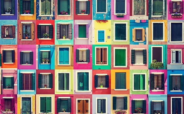
# Setup our parameters
width = 1920
height = 1080
picture_path = 'picture.png'
result_path = 'results.png'
blocks_per_grid = (512, 512)
threads_per_block = (16, 16)


# Initialize our arrays
canvas = make_complex_canvas(width, height)
mapped = np.zeros_like(canvas)
image = plt.imread(picture_path)
out = np.zeros((height, width, image.shape[2]), dtype=image.dtype)

# Send the arrays to the GPU
gpu_canvas = cuda.to_device(canvas)
gpu_mapped = cuda.to_device(mapped)
gpu_image = cuda.to_device(image)
gpu_out = cuda.to_device(out)

# call the wallpaper function
example_wallpaper[blocks_per_grid, threads_per_block](gpu_mapped, gpu_canvas)

# Bring it back to the CPU
mapped = gpu_mapped.copy_to_host()

# Get the range for the colormap
x_min = np.amin(np.abs(mapped))
x_max = np.amax(np.abs(mapped))
y_min = np.amin(np.angle(mapped))
y_max = np.amax(np.angle(mapped))

# call the colormap function
colormap_complex[blocks_per_grid, threads_per_block](gpu_out, gpu_mapped, gpu_image, x_min, x_max, y_min, y_max)

plt.imsave(result_path, gpu_out.copy_to_host())